The ALASKA Benchmark is an end-to-end benchmark for Big Data Integration tasks. ALASKA Datasets are organized into product category verticals. For each vertical we provide:
- product specifications extracted from web pages collected from different sources;
- original web pages;
- manually curated labelled data related to different integration tasks.
The ALASKA Benchmark supports the following integration tasks:
- Entity Resolution
- Schema Alignment
- Knowledge Graph Construction
- Valter Crescenzi (Roma Tre University)
- Andrea De Angelis (Roma Tre University)
- Xin Luna Dong (Amazon Research)
- Donatella Firmani (Roma Tre University)
- Maurizio Mazzei (Roma Tre University)
- Paolo Merialdo (Roma Tre University)
- Federico Piai (Roma Tre University)
- Divesh Srivastava (AT&T Labs-Research)
News
- 2019-12-23: Entity Resolution challenge starts. New
- 2019-12-19: Datasets for CAMERA and MONITOR verticals released.
Table of Contents
1. Product specification datasets
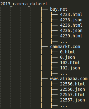
The ALASKA Benchmark datasets consist of HTML web pages, collected from different web sources, and JSON extracted product specifications. You can download our datasets from the Downloads section.
Example of product specification
{

 "<page title>": "Samsung Smart WB50F Digital Camera White Price in India with Offers & Full Specifications | PriceDekho.com",

 "brand": "Samsung",

 "dimension": "101 x 68 x 27.1 mm",

 "display": "LCD 3 Inches",

 "pixels": "Optical Sensor Resolution (in MegaPixel)\n16.2 MP"

  "battery": "Li-Ion"

}
Product specifications we have collected have the following properties:
- they contain (attribute_name, attribute_value) pairs;
- the <page title> attribute is always present;
- the set of attribute names which are available in specifications can have considerable heterogeneity, both intra source and across sources (schema heterogeneity);
- the set of attribute values which are associated with the same attribute name can have considerable heterogeneity, both intra source and across sources (attribute values heterogeneity);
- different sources (and also the same source) could use different attribute names (or values) to describe the same concept (attrubute synonymy, e.g. "resolution" and "pixels");
- the same attribute name (or value) could be used to describe different concepts (attribute homonymy, e.g. "battery" that can refer to "battery type", like "AAA", or "battery chemistry", like "Li-Ion").
In the following sections we will present our datasets, providing a pre-integration profiling.
- CAMERA
- MONITOR
1.1 CAMERA vertical
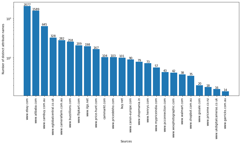
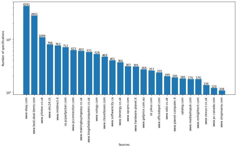
CAMERA dataset contains 29,787 specifications collected from 24 web sources. The specifications contain ~4.6k distinct attribute names.
- Figure 1 shows the sources of the CAMERA dataset on the x axis and the number of specifications on the y axis.
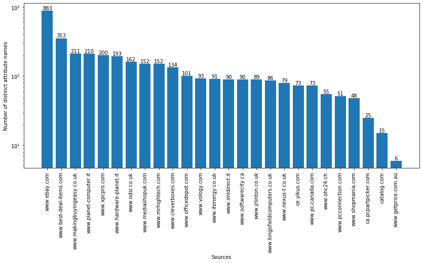
- Figure 2 shows the sources of the CAMERA dataset on the x axis and the number of distinct attribute names on the y axis.
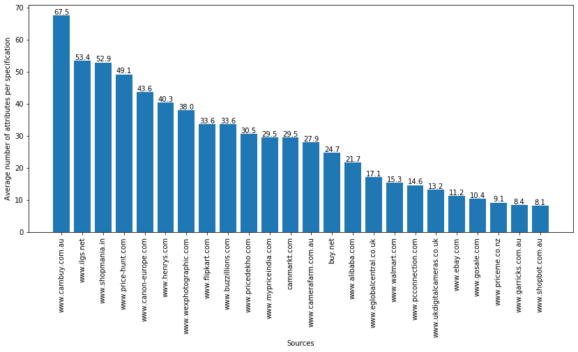
- Figure 3 shows the sources of the CAMERA dataset on the x axis and the average number of attributes inside specifications on the y axis.
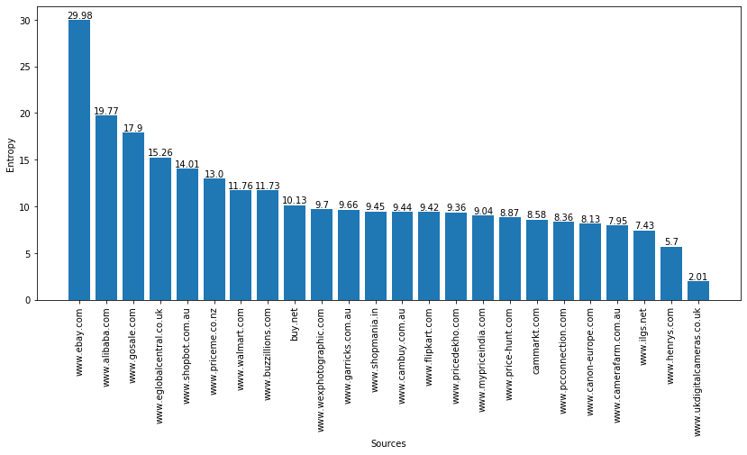
- Figure 4 shows the sources of the CAMERA dataset on the x axis and the schema entropy on the y axis. Entropy is calculated using the following formula: \[H(x) = - \sum_i{p(x_i) * log_2(p(x_i))} \] where the symbol \(x_i\) represents a bit-vector of the attribute names present in the specifications of a source. For instance, source www.ebay.com uses a very different set of attribute names in its specifications (high entropy), while www.ukdigitalcameras.co.uk uses a homogeneous set of attribute names in its specifications.
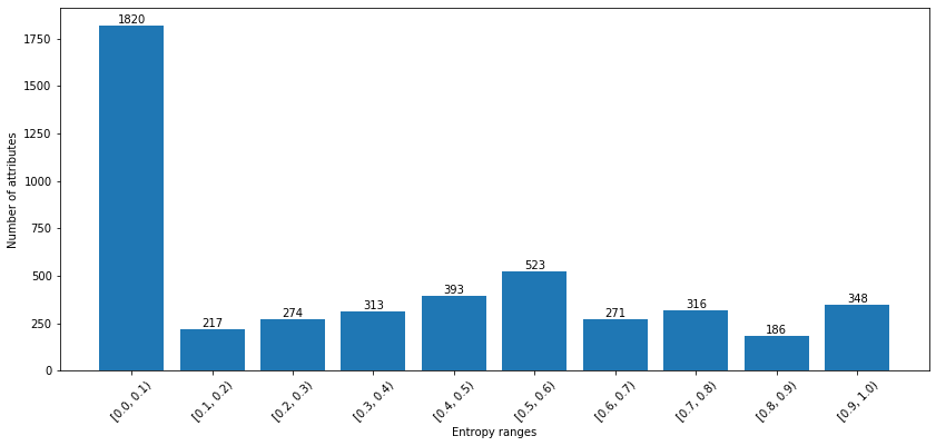
- Figure 5 shows the entropy range (normalized between 0 and 1) on the x axis and the number of attribute names on the y axis. Entropy is calculated on the attribute values using the following formula: \[H(x) = - \sum_i{p(x_i) * log_2(p(x_i))} \] where the symbol \(x_i\) represents the entire string of the attribute value. For instance, 348 attribute names have a very large set of distinct values (high entropy), while 1820 attribute names have a low number of possible values. In this range we also have attributes with few distinct values, such as yes/no.
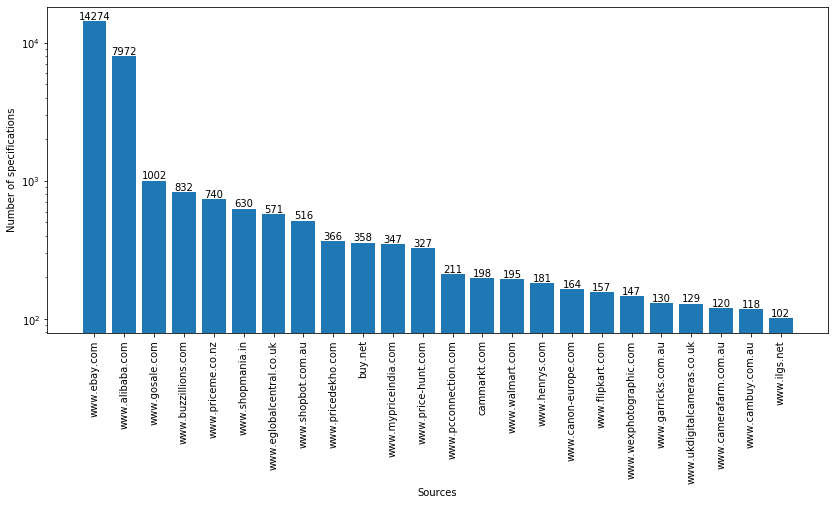
The CAMERA datasets contains 2 head (i.e. with a high number of specifications) sources and 22 tail (i.e., with a medium/low number of specifications) sources.
1.2 MONITOR vertical
MONITOR dataset contains 16,662 specifications collected from 26 web sources. Specifications contains ~3.7k distinct attribute names.
- Figure 1 shows the sources of the MONITOR dataset on the x axis and the number of specifications on the y axis.
- Figure 2 shows the sources of the MONITOR dataset on the x axis and the number of distinct attribute names on the y axis.
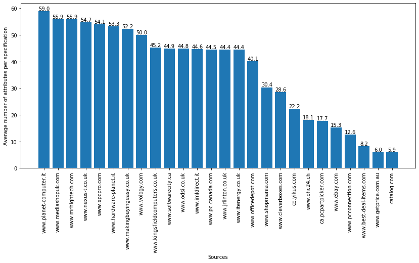
- Figure 3 shows the sources of the MONITOR dataset on the x axis and the average number of attributes inside specifications on the y axis.
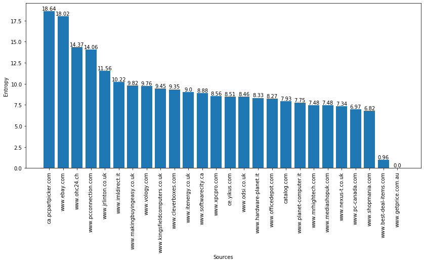
- Figure 4 shows the sources of the MONITOR dataset on the x axis and the schema entropy on the y axis. Entropy is calculated using the following formula: \[H(x) = - \sum_i{p(x_i) * log_2(p(x_i))} \] where the symbol \(x_i\) represents a bit-vector of the attribute names present in the specifications of a source. For instance, source www.ca.pcpartpicker.com uses a very different set of attribute names in its specifications (high entropy), while www.getprice.com.au uses the same set of attribute names in all its specifications (schema homogeneity).
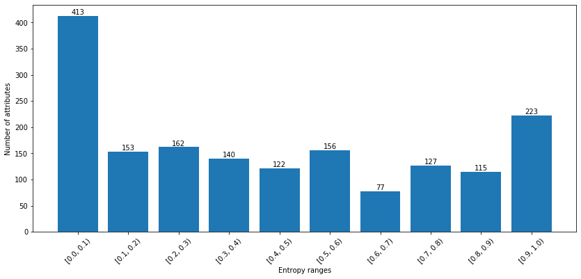
- Figure 5 shows the entropy range (normalized between 0 and 1) on the x axis and the number of attribute names on the y axis. Entropy is calculated on the attribute values using the following formula: \[H(x) = - \sum_i{p(x_i) * log_2(p(x_i))} \] where the symbol \(x_i\) represents the entire string of the attribute value. For instance, 223 attribute names have a very large set of distinct values (high entropy), while 413 attribute names have a low number of possible values. In this range we also have attributes with few distinct values, such as yes/no.
The MONITOR datasets contains 2 head (i.e. with a high number of specifications) sources and 24 tail (i.e., with a medium/low number of specifications) sources.
2. Labelled Data
We manually curated an extensive collection of labelled representative samples for each task in the ALASKA benchmark.
2.1 Entity Resolution task
For the Entity Resolution task we needed to identify which specifications represents the same real-world entity (e.g. Canon EOS D50).
The methodology we used to creating the Entity Resolution ground truth is the following:
- estimate the entity size distribution extracting the model ID from the specifications (e.g. D50);
- partition entities into 3 categories: head, middle and tail, based on the number of specifications and sources involved in the cluster (where a cluster represents an entity);
- pick a certain number of clusters (or entities) by stratified sampling on the above categories;
- select a specification to be used as a seed for each cluster selected at the previous step;
- find all the specifications referring to the same real-world entity of the seeds by crowdsourcing matching/non-matching pairs.
We provide as labelled data random subsets of the above ground truth with different size, dubbed SMALL, MEDIUM, LARGE and X-LARGE
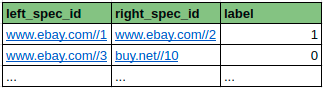
.Each dataset is provided in a CSV format with three columns: "left_spec_id", "right_spec_id" and "label".
The "spec_id" is a global identifier for a specification and is the concatenation of the source name with the json number of the specification, separated by a special character "//" (e.g. "www.ebay.com//1000" is the global identifier for the 1000.json file inside www.ebay.com directory).
Each row of the CSV file represents a pair of specifications. Label=1 means the row is a matching pair, whereas label=0 means the row is a non matching pair.
The methodology to create such labelled sets is the following:
- consider a graph where the nodes are the specifications we have labelled and the edge between two nodes is weighed based on the label (=1 for matching pairs, =0 for non-matching pairs). This graph has a connected component for each labelled entity;
- select a certain number of connected components (entities) randomly;
- select a certain percentage of specifications from each connected component (CC) selected at point 2;
- for each CC:
- consider the clique consisting of the specifications selected at point 3 for that CC. All these edges are matching pairs for the labelled set;
- consider the Cartesian product between the instances of that CC and all the remaining CCs. All these edges are non-matching pairs for the labelled set;
N.B. Every larger labelled set includes the smaller ones (e.g. the LARGE labelled set includes the SMALL and the MEDIUM).